Why REW (and why it's free)
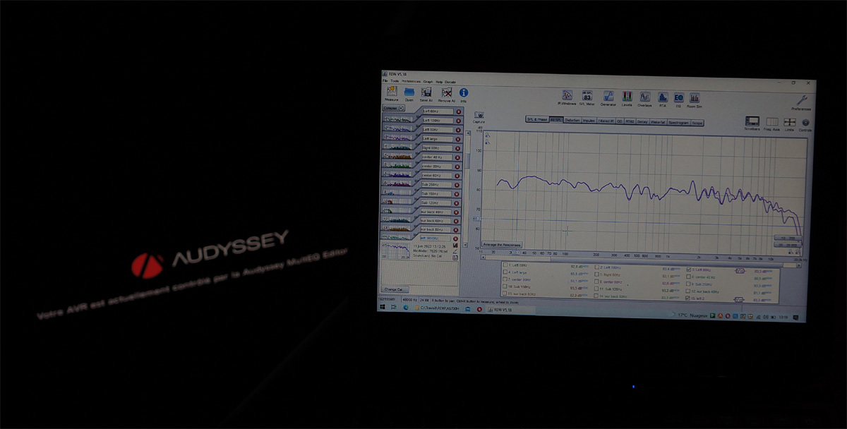
REW measures your room's real response: frequency response, reverberation time (RT60), room modes, waterfall, distortion… It's the free, cross-platform community reference. HTM doesn't replace it: it predicts before the build, then imports your REW measurements to validate the prediction, or correct it, seat by seat.
Home cinema or studio? Same approach: whether you're designing an immersive multichannel room or a nearfield stereo setup (monitoring / hi-fi), you measure, import, and let HTM analyse. HTM even accounts for the listening regime, whether near field, mid field or far field. Just adapt the mic's distance and position to your case.
The mic: go for a UMIK-1 / UMIK-2
A calibrated USB measurement mic is the simplest option: it plugs in over USB, with no interface or preamp. The de-facto standard is the miniDSP UMIK-1 (or the newer UMIK-2), and this guide is built around it. Each unit ships with its individual calibration file, downloaded from miniDSP's site using the serial number engraved on the mic.
- A UMIK-1 / UMIK-2 and its stand (tripod), at ear height.
- REW installed (free), from roomeqwizard.com.
- A link from the PC to your system (HDMI to the amp / processor) to play the sweep on the chosen channel.
The two calibration files: 0° and 90°
Often overlooked, yet decisive for accuracy: the UMIK ships with two calibration files, and you must load the right one depending on how you orient the mic.
- The "90°" file, mic pointed at the ceiling (vertical). This is the one for room measurements at the listening position: sound arrives from everywhere (speakers + reflections) and the mic captures that diffuse field. Use it for all your measurements at the various listening positions, the ones HTM analyses.
- The "0°" file, mic pointed horizontally, straight at the speaker (on-axis). This is the one for measuring a single speaker on-axis / near-field, when you aim directly at a driver.
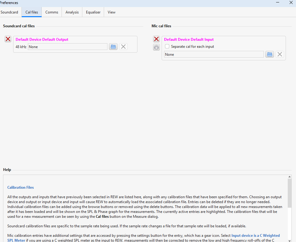
Load it under Preferences → Cal files → Mic cal files. In practice, to prepare a file for HTM you'll mostly stay on the 90° file, mic vertical at the listening position.
Set up REW
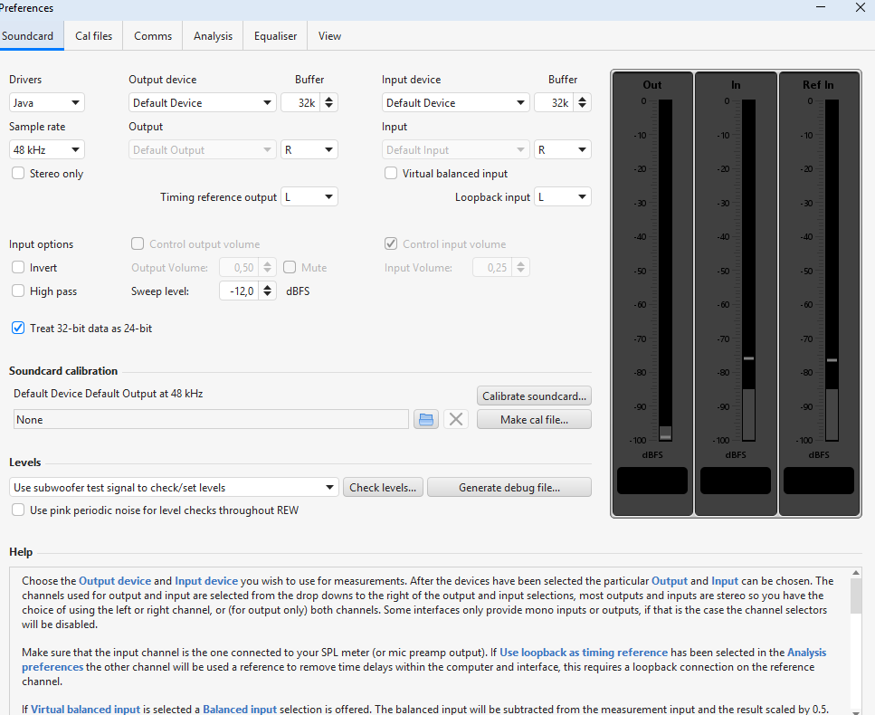
In Preferences → Soundcard, choose the output that feeds your system and the input = the UMIK. Check the sample rate (48 kHz), then run a level check (Check levels) to avoid clipping. Set a safe listening level, identical between measurements (REW's SPL tab helps you aim for ~75 dB).
Where to place the mic and what to measure
File quality comes first from mic placement:
- Mic on a stand, at ear height, at the main listening position (MLP), the central seat first.
- Mic vertical (90° file), head clear, away from an armrest or backrest that would create a stray reflection.
- Then repeat at each seat you want to optimise: HTM then compares position by position.
One clean sweep per seat beats ten sloppy measurements: these are the curves HTM will analyse.
Two habits that change everything: measure at exactly the same spot before and after a change (otherwise the curves aren't comparable). Then, to avoid measuring your own body, start the sweep with a short delay ("Delay") so you can step aside. The listening position must stay clear. Measuring distance follows your listening regime: closer in the near field, further back in the far field.
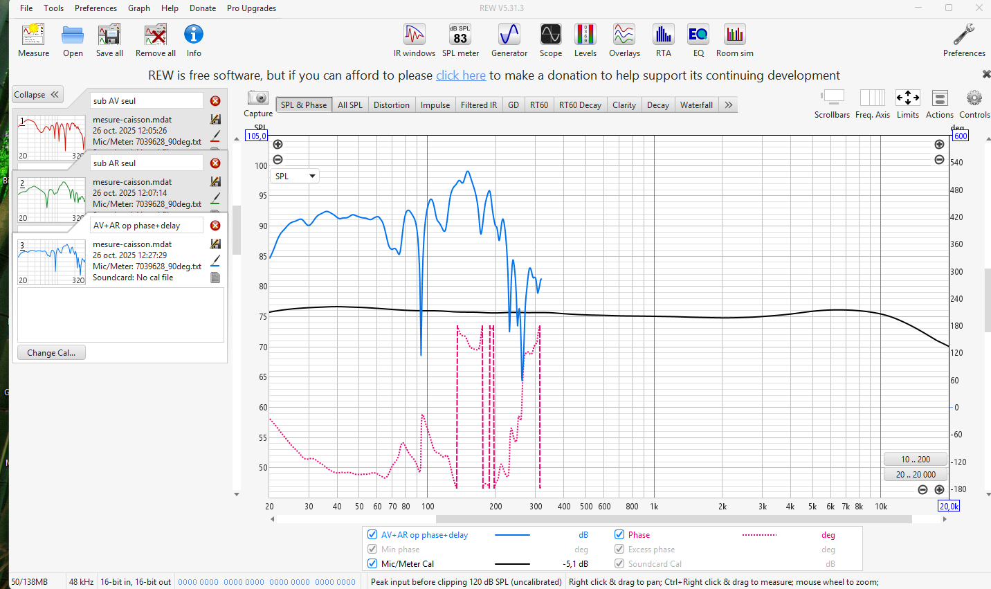
The moving-mic trick (the "MMM"). MMM stands for Moving Mic Method, literally "the method where you move the mic". The idea is simple: instead of leaving the mic still on its stand, you play a continuous signal and slowly sweep the mic around the head (within about a 50 cm radius) while REW averages what it picks up. The result irons out the small point-to-point variations and gives a very stable curve, ideal to judge the overall tonal balance of a listening zone or to dial in a subwoofer. Still, keep fixed, channel-by-channel measurements alongside (mic held still): those are what HTM uses for distances, levels and per-speaker EQ.
Locating your listening regime. What matters here is the critical distance: the point where the speaker's direct sound and the room's reverberant field become roughly equal. (Strictly, that is related to, but not the same as, the acoustic near-field / far-field boundary, which also depends on the source's size and the wavelength; for choosing a listening distance, though, the critical distance is the useful marker.) To find it, measure while backing away in steps (~50 cm) from the speaker: as long as the level clearly drops as you retreat, the direct sound dominates. Once it steadies, the room has taken over. Set the measuring distance (and the regime declared in HTM) accordingly.
Measure each channel (multichannel or stereo)
For a real multichannel room, don't stop at "left + right". Measure each speaker separately: the Centre, Surrounds, rears, ceiling speakers (Atmos), sub(s), playing the sweep through one channel at a time and naming each measurement by its channel (L, C, R, SL, SR, Top…). REW routes the sweep to the chosen channel. On the amp side, isolate the channel being measured.
For stereo / studio listening, the same logic applies, more simply: measure L alone, R alone, then L+R together: the three, measured separately, help reveal a phase problem between the two speakers.
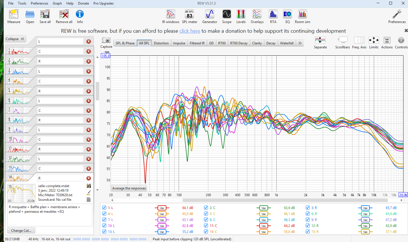
You end up with one measurement per channel (and per seat). Overlaid, they give a whole-room view, and above all HTM derives distances, levels, crossovers and a per-channel EQ from them.
Reading the values: what's good, what's to improve
The frequency response shows dips and peaks: in the bass they reveal the room modes. Higher up, they depend mostly on placement and treatment. Reading tip: apply some smoothing (1/12 to 1/48 octave, Graph → Smoothing menu) to bring out the trends without the fine noise.
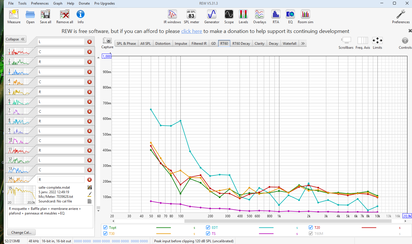
The RT60 (reverberation time per band) is read against a target. In the example below, above ~300 Hz the RT60 is short and steady (~0.1–0.15 s): the room is well damped and quite dry (whether that is ideal depends on the room's use and your target). Below ~100 Hz it climbs toward 0.4–0.6 s: the bass rings on, the band to improve (typically with bass traps). The goal is a fairly flat RT60, neither too long ("cavernous" sound) nor too dead. The target depends on the use: rather dry for a studio / monitoring room (≈ 0.3 s), a bit more lively for a home cinema. In a small room, conventional RT60 becomes unreliable in the bass, where the field is not diffuse: REW's Topt estimator helps find a usable decay slope when one exists, but below the Schroeder frequency, read the decay, waterfall and spectrogram rather than treating RT60 as a diffuse-field value.
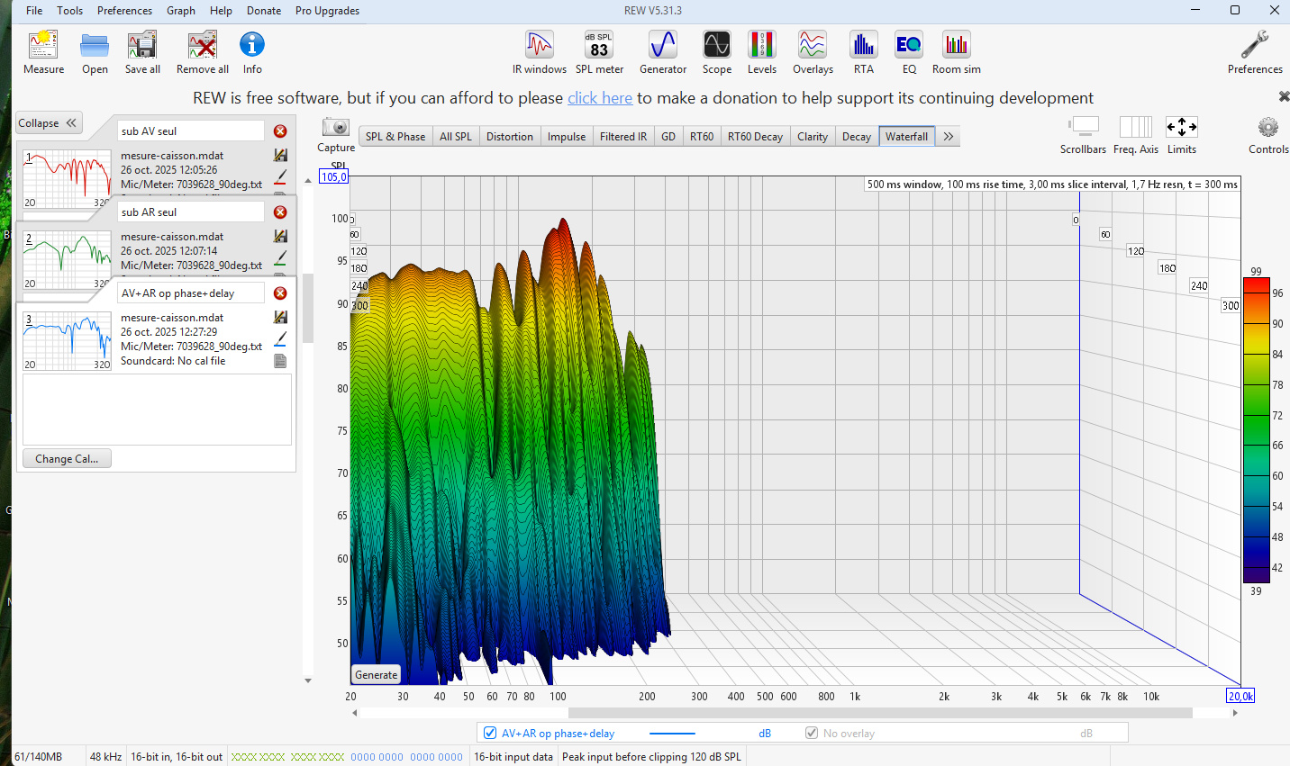
The waterfall visually confirms which resonances ring on over time.
Finally, the ETC curve (Filtered IR tab) shows how energy decays over time and brings out the early reflections just after the direct sound. Spot the ones that rise too high: a strong reflection smears the stereo image. Tip: the delay gives the reflection's extra path length (≈ 340 m/s × time), not the wall's distance itself; the actual mirror point to treat depends on the speaker / listener / wall geometry (HTM computes it for you). The ETC also shows the estimators (Topt, EDT, C50/C80 clarity).
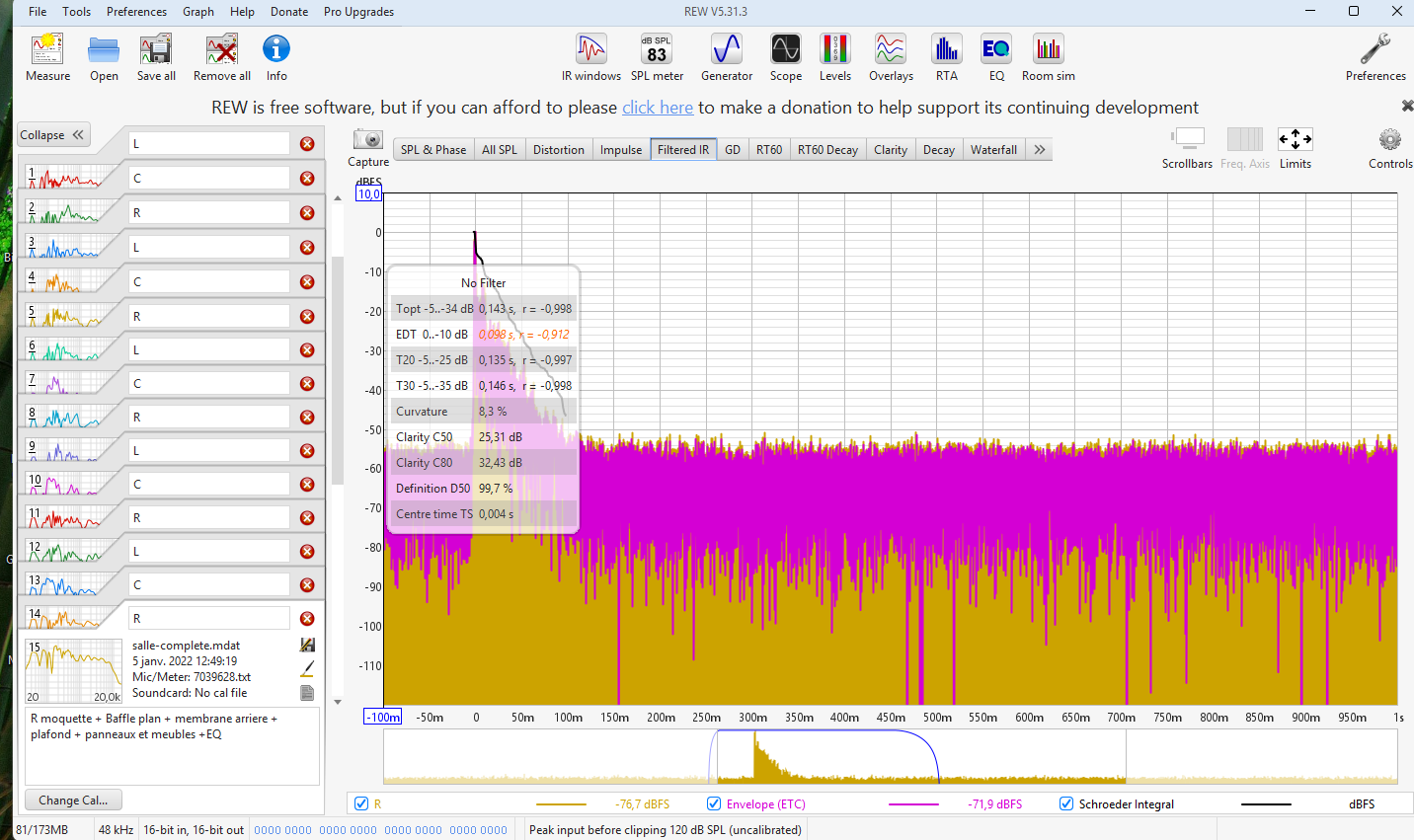
Not all reflections are equal. The very first ones (less than ~10–15 ms after the direct sound, a boundary a few metres away) are largely fused by the ear with the direct sound (precedence / Haas effect), so they disturb localisation less than later ones. They are not harmless, though: even fused, a strong early reflection still colours the timbre and can comb-filter the response, which is why treating the first reflection points helps. It's the later, stronger reflections, returning clearly detached, that need treating. Aim for a clean decay right after the peak (on the order of −20 dB within the first tens of milliseconds). To locate a specific reflection, REW's wavelet spectrogram is even easier to read than the ETC.
Correcting: cut peaks first, fill dips almost never
Once the room is measured, the temptation is to "flatten" everything with EQ. The right instinct is the opposite: shave the peaks, don't fill the dips. A deep bass dip is almost always a modal cancellation (two waves opposing each other at the seat): boosting it with EQ wastes amplifier headroom and, in a non-minimum-phase zone, doesn't even fill in. A +8 dB correction can yield less than 8 dB real at the mic. Cutting a peak, on the other hand, is effective and safe.
Bass problems (modes, dips) are solved first by placement (of the speaker, the sub and the seat) and by passive treatment (bass traps). EQ only comes in for the finish. As an expert thread puts it: "electronic correction is no substitute for optimised placement." That's exactly HTM's logic: predict and optimise placement first, measure next, correct last.
Export for HTM
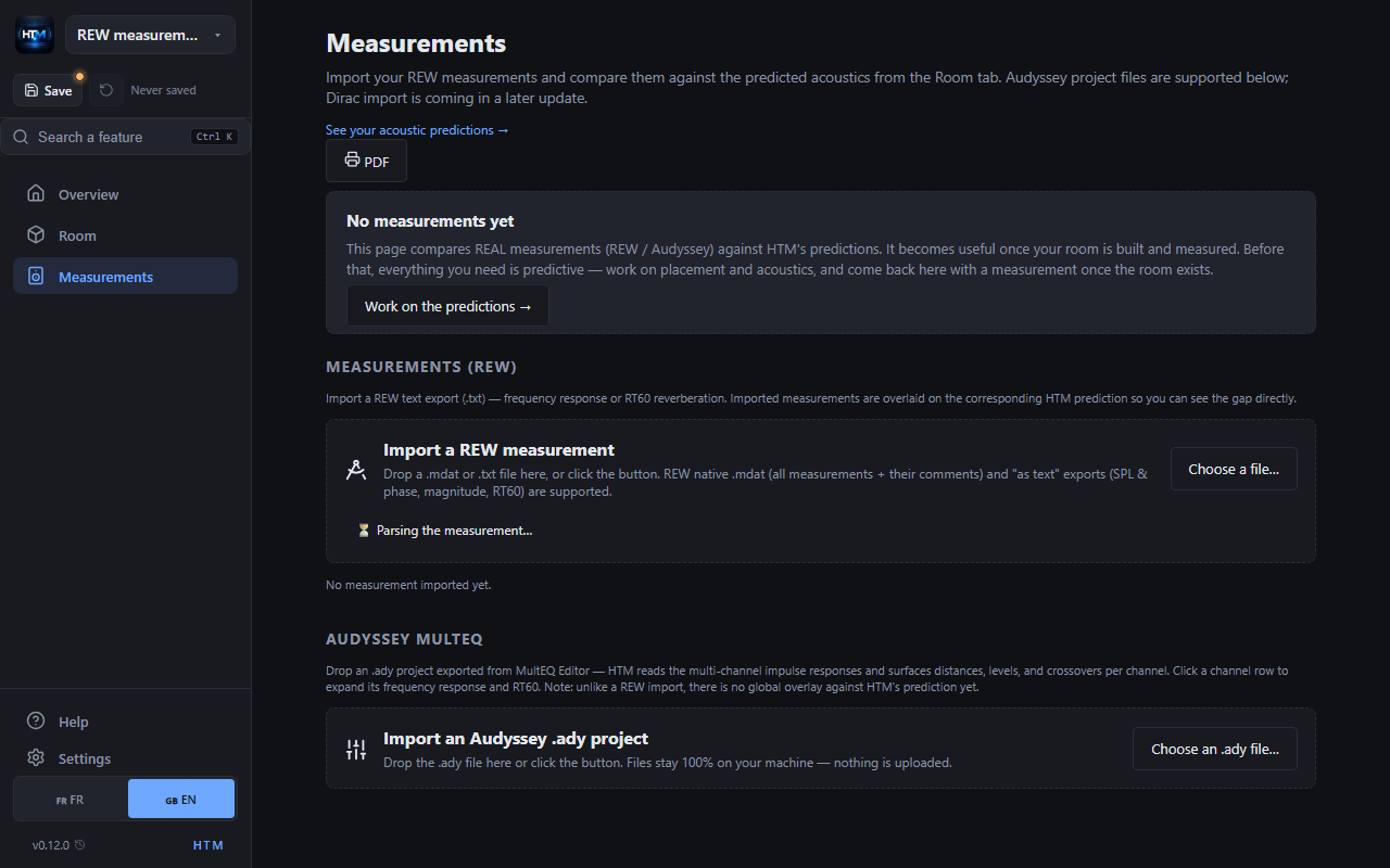
Save the REW project as .mdat (native, recommended) or export each measurement as text. Those are the two formats HTM imports.